The Central Limit Theorem (CLT) is a fundamental concept in statistics and an essential tool in biostatistics. It provides a foundation for understanding how sample data can be used to make inferences about an entire population. This article will guide students through the development and significance of the CLT, exploring the role of sample means, population means, and the measures of dispersion—particularly the standard error (SE), standard deviation (SD), and confidence interval (CI).
The Origins of the Central Limit Theorem
The CLT emerged in the 18th century through the work of mathematicians like Abraham de Moivre and Pierre-Simon Laplace. De Moivre, while studying probabilities in games of chance, observed that repeated trials formed a bell-shaped distribution. Laplace expanded on this by demonstrating that the sum of independent random variables approximates a normal distribution as the sample size increases. This was a profound realization because it showed that even non-normally distributed data could produce a predictable distribution of means.
Later, Carl Friedrich Gauss solidified the concept of the normal distribution while studying measurement errors in astronomy. Gauss observed that when repeated measurements are taken, the errors typically form a bell-shaped curve. This normal distribution became the foundation for much of statistical analysis, allowing researchers to describe and predict patterns in data.
How the Central Limit Theorem Works
The CLT states that, for a sufficiently large sample size, the distribution of sample means will approximate a normal distribution regardless of the original population’s distribution. This result is powerful because it allows us to use a sample mean as an estimate for the population mean, even when we don’t know the distribution of the underlying data.
In practical terms, the CLT explains why the mean of a sample often provides a reliable estimate of the population mean. As we increase the sample size, the sample mean will tend to get closer to the true population mean, creating the basis for inferential statistics.
Understanding Central Tendency and Dispersion
To make inferences about a population, we need to understand central tendency (mean, median, mode) and dispersion (SD, SE, CI). Central tendency measures provide a summary of where most data points fall, while dispersion measures show how spread out the data points are.
• Mean: The average value of the data points, highly sensitive to outliers.
• Median: The middle value in a sorted dataset, less affected by extreme values.
• Mode: The most frequently occurring value, useful for identifying common outcomes.
In medical research, choosing the correct central tendency measure is important. For instance, in analyzing cholesterol levels among patients, the median might offer a more accurate “central” measure than the mean if the dataset contains extreme outliers.
Measures of Dispersion: SD, SE, and CI
Understanding variability is essential in research, as it indicates how consistent or spread out data points are around the mean. Here’s how SD, SE, and CI are applied:
• Standard Deviation (SD): This measures the spread of data within a sample. A high SD means individual values vary widely around the mean, while a low SD means values cluster closely around the mean.
• Standard Error (SE): This measures how much the sample mean is expected to deviate from the true population mean. The SE decreases as sample size increases, reflecting that larger samples provide more precise estimates of the population mean.
• Confidence Interval (CI): This gives a range within which the population mean likely falls. A 95% CI means we are 95% confident that the interval contains the true population mean. CIs allow researchers to report not only an estimate but also the reliability of that estimate.
Interpreting “Small” SE and CI
What constitutes a “small” SE or CI depends on several factors:
1. Relative Size to the Mean: Typically, an SE or CI that is within 5-10% of the mean can be considered precise in many fields. For example, if the mean blood pressure reduction in a study is 10 mmHg, an SE between 0.5 and 1 mmHg would be considered precise because it reflects only a small percentage (5-10%) of the mean value.
2. Clinical Relevance: In medicine, a small SE or narrow CI must also be clinically meaningful. A small SE that doesn’t offer insight into a meaningful treatment effect wouldn’t necessarily be useful.
3. Sample Size and Precision: SE decreases as sample size increases. Larger samples reduce SE, resulting in narrower CIs, and provide more reliable estimates of the population mean.
Proving Standard Error with R Simulation
To demonstrate that SE accurately represents the precision of the sample mean, we can use a simulation. Here’s an R script that simulates a population, repeatedly samples it, and shows that the simulated SE (standard deviation of sample means) approximates the theoretical SE:
# Load necessary libraries
library(dplyr)
library(gt)
# Set parameters for population
population_mean <- 120 # Hypothetical population mean (e.g., blood pressure)
population_sd <- 15 # Hypothetical population standard deviation
population_size <- 100000 # Large population size for accurate simulation
num_samples <- 1000 # Number of samples to draw per sample size
# Generate a large population
set.seed(42)
population_data <- rnorm(population_size, mean = population_mean, sd = population_sd)
# Define different sample sizes for comparison
sample_sizes <- c(10, 50, 100, 500, 1000)
# Create a data frame to store results
results <- data.frame(Sample_Size = integer(),
Mean_of_Sample_Means = numeric(),
Simulated_SE = numeric(),
CI_Lower_Bound = numeric(),
CI_Upper_Bound = numeric())
# Loop through each sample size and calculate metrics
for (sample_size in sample_sizes) {
# Draw multiple samples and calculate mean for each sample
sample_means <- replicate(num_samples, mean(sample(population_data, sample_size, replace = FALSE)))
# Calculate the mean of sample means, simulated SE, and CI bounds
mean_of_sample_means <- mean(sample_means)
simulated_se <- sd(sample_means)
ci_lower_bound <- mean_of_sample_means - 1.96 * simulated_se
ci_upper_bound <- mean_of_sample_means + 1.96 * simulated_se
# Store the results in the data frame
results <- results %>% add_row(Sample_Size = sample_size,
Mean_of_Sample_Means = mean_of_sample_means,
Simulated_SE = simulated_se,
CI_Lower_Bound = ci_lower_bound,
CI_Upper_Bound = ci_upper_bound)
}
# Display the results table using gt for a neat format
results %>%
gt() %>%
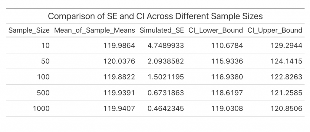
tab_header(title = "Comparison of SE and CI Across Different Sample Sizes")
The output of this simulation with different sample sizes illustrates how SE and CI change with sample size:
Explanation of Results
In this simulation:
• The mean of the sample means should be close to the population mean, confirming that sample means provide a reliable estimate of the true mean.
• The standard deviation of the sample means (simulated SE) will approximate the theoretical SE, supporting that SE reflects how much the sample mean varies from the population mean.
• The decreasing SE and narrowing CI with increasing sample size illustrate that larger samples improve the precision of the sample mean.
Application in Medical Research
In medical research, these measures of dispersion are vital. For instance, in a clinical trial, researchers might measure the mean reduction in blood pressure after a treatment. Reporting the mean reduction alone isn’t enough; they also report SE and CI to show the precision and reliability of this estimate. A smaller SE suggests the sample mean closely approximates the true effect in the population, while the CI gives a range within which the true effect likely falls.
Summary
The Central Limit Theorem and measures like SD, SE, and CI form the statistical backbone of medical research. Through understanding these concepts, researchers can confidently use sample data to estimate population parameters, assess data reliability, and make evidence-based decisions in healthcare.
Disclaimer
This article was created using ChatGPT for educational purposes and should not replace professional statistical advice.